Antarctic Oscillation Index [AAO index]
Teleconnective indices: Antarctic Oscillation Index [AAO index]
The
It is a climate driver for Australia, influencing the country's weather conditions –
It is associated with storms and cold fronts that move from west to east that bring
precipitation to southern Australia.
In its positive phase (AAO+), the westerly wind belt that drives the
Antarctic Circumpolar Current intensifies and contracts towards Antarctica. In winter, a
positive phase increases rainfall (including East coast lows) in south-eastern Australia
(above Victoria) due to higher onshore flows from the Pacific Ocean, decrease rain in the south-west,
and decrease snow in the alpine areas. In spring and summer, a positive phase reduces the chance
of extreme heat and increases humid onshore flows, therefore making spring and summer more wetter
than normal. A positive phase would usually occur more frequently with a La Niña event.
Its negative phase involves the belt moving towards the equator, whereby decreasing
rainfall in the southeast of Australia in the summer and as well as raising the possibility
of spring heatwaves. Moreover, winters will usually be wetter than normal in the south
and southwest with more snowfall in the alpine areas, but drier in the east coast due to less
moist onshore flows from the east and blockage of cold fronts by the Great Dividing Range,
which would act as a rain shadow. This phase will usually be more frequent with an
El Niño event.
Credits: cpc.ncep.noaa.gov
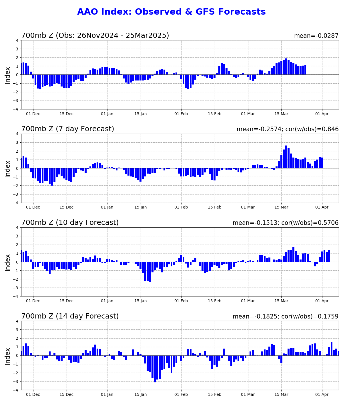
AAO index: observed & GFS forecasts
The daily AAO indices are shown for the previous 120 days, and the GFS forecasts of the daily AAO index at selected lead times are appended onto the time series. The indices are standardized by standard deviation of the observed monthly AO index from 1979-2000. A 3-day running mean is applied to the forecast time series.
Credits: cpc.ncep.noaa.gov
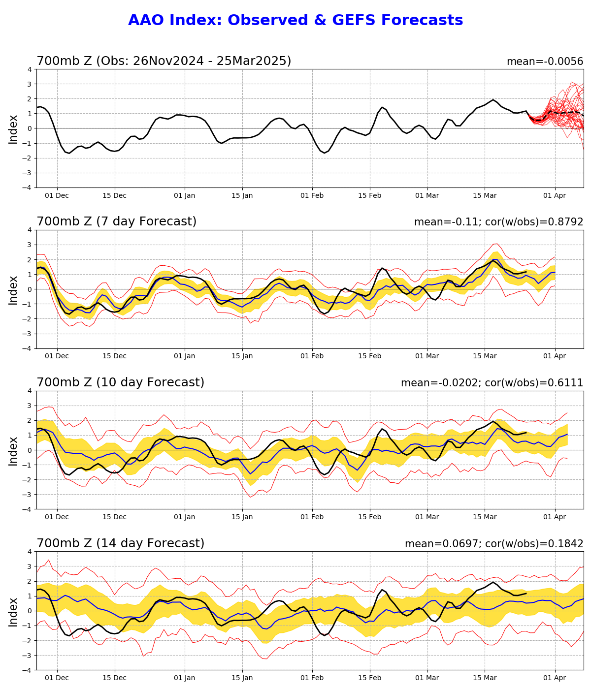
AAO index: observed & GFS Ensemble forecasts
The daily AAO indices are shown for the previous 120 days, and the ensemble forecasts of the
daily AAO index at selected lead times are appended onto the time series. The indices are standardized
by standard deviation of the observed monthly AAO index from 1979-2000. A 3-day running mean is applied
to the forecast time series.
The values at the upper left and right corners of each figure indicate the mean value of the AAO
index and the correlation coefficients between the observations and the forecasts, respectively.
The first panel shows the observed AAO index (black line)
plus forecasted AAO indices from each of the
11 MRF ensemble members starting from the last day of the observations
(red lines).
The ensemble mean forecasts of the AAO index are obtained by averaging
the 11 MRF ensemble
members (blue lines), and the observed AAO index (black line)
is superimposed on each panel for comparison.
For the forecasted indices (lower 3 panels), the yellow shading
shows the ensemble mean plus and
minus one standard deviation among the ensemble members, while the upper and lower
red lines show
the range of the forecasted indices, respectively.
Credits: cpc.ncep.noaa.gov
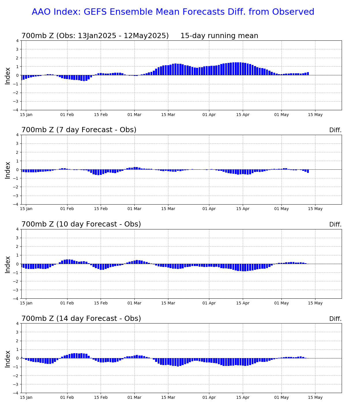
AAO index: GFS Ensemble mean forecasts differences from observed
Differences between 15-day running mean values of AAO index observation and the Ensemble mean outlooks.
Credits: cpc.ncep.noaa.gov
Monthly mean AAO index since January 1979
In the following table all the average monthly values of the AAO index from 1950 to today.
With a red scale, values higher than +0.5 are highlighted, with a blue scale those lower than -0.5.
Below the table, a diagram again shows the AAO values recorded so far.
| JAN | FEB | MAR | APR | MAY | JUN | JUL | AUG | SEP | OCT | NOV | DEC | |
|---|---|---|---|---|---|---|---|---|---|---|---|---|
| 1979 | +0.209 | +0.356 | +0.899 | +0.678 | +0.724 | +1.700 | +2.412 | +0.545 | +0.629 | +0.160 | -0.422 | -0.951 |
| 1980 | -0.447 | -0.980 | -1.424 | -2.068 | -0.479 | +0.286 | -1.944 | -0.997 | -1.701 | +0.577 | -2.013 | -0.356 |
| 1981 | +0.231 | +0.039 | -0.966 | -1.462 | -0.344 | +0.352 | -0.986 | -2.118 | -1.509 | -0.260 | +0.626 | +1.116 |
| 1982 | -0.554 | +0.277 | +1.603 | +1.531 | +0.118 | +0.920 | -0.415 | +0.779 | +1.580 | -0.702 | -0.849 | -1.934 |
| 1983 | -1.340 | -1.081 | +0.166 | +0.149 | -0.437 | -0.263 | +1.114 | +0.792 | -0.696 | +1.194 | +0.727 | +0.475 |
| 1984 | -1.097 | -0.544 | +0.251 | -0.204 | -1.237 | +0.426 | +0.890 | -0.548 | +0.327 | -0.009 | -0.024 | -1.476 |
| 1985 | -0.795 | +0.215 | -0.134 | +0.032 | -0.066 | -0.331 | +1.914 | +0.595 | +1.507 | +0.471 | +1.085 | +1.240 |
| 1986 | +0.158 | -1.588 | -0.770 | -0.087 | -1.847 | -0.619 | +0.089 | -0.157 | +0.849 | +0.306 | -0.223 | +0.886 |
| 1987 | -0.950 | -0.708 | -0.133 | -0.286 | +0.039 | -0.702 | -1.531 | +1.485 | -0.799 | +0.456 | +1.060 | +0.272 |
| 1988 | -0.612 | +0.551 | -0.219 | -0.077 | -0.749 | -1.055 | +0.576 | -0.745 | -0.689 | -2.314 | +0.401 | +1.075 |
| 1989 | +0.618 | +0.849 | +0.632 | -0.573 | +2.691 | +1.995 | +1.458 | -0.132 | -0.121 | +0.136 | +0.572 | -0.445 |
| 1990 | -0.352 | +1.151 | +0.414 | -1.879 | -1.803 | +0.093 | -1.215 | +0.466 | +1.482 | +0.139 | -0.359 | -0.312 |
| 1991 | +0.869 | -0.852 | +0.522 | -0.639 | -0.539 | -1.155 | -1.220 | +0.035 | -0.513 | -0.623 | -0.804 | -2.067 |
| 1992 | +0.073 | -1.627 | -1.010 | -0.439 | -2.032 | -2.193 | -0.566 | -0.349 | +0.435 | -0.319 | +0.122 | +0.244 |
| 1993 | -2.021 | +0.437 | -0.378 | +0.087 | +1.260 | +1.218 | +1.957 | +1.083 | +1.061 | +0.748 | +0.324 | +1.028 |
| 1994 | +0.723 | +1.157 | +0.693 | -0.052 | -0.153 | -1.682 | -0.492 | +1.910 | -0.947 | -0.578 | -0.793 | +0.933 |
| 1995 | +1.448 | +0.533 | -0.154 | +0.649 | +1.397 | -0.802 | -3.010 | -0.697 | +1.173 | -0.057 | +0.143 | +1.470 |
| 1996 | +0.332 | -0.525 | +0.543 | +0.115 | +0.983 | -0.252 | +0.021 | -1.502 | -1.314 | +0.966 | -1.667 | -0.023 |
| 1997 | +0.369 | -0.244 | +0.701 | -0.458 | +1.028 | -0.458 | +0.780 | +0.768 | +0.122 | -0.595 | -1.905 | -0.836 |
| 1998 | +0.412 | +0.390 | +0.736 | +1.927 | -0.038 | +1.031 | +1.450 | +0.904 | -0.122 | +0.400 | +0.817 | +1.435 |
| 1999 | +0.999 | +0.456 | +0.180 | +0.949 | +1.639 | -1.325 | +0.316 | +0.042 | -0.012 | +1.653 | +0.901 | +1.784 |
| 2000 | +1.273 | +0.620 | +0.133 | +0.233 | +1.127 | +0.117 | +0.059 | -0.673 | -1.853 | +0.347 | -1.537 | -1.290 |
| 2001 | -0.471 | -0.265 | -0.555 | +0.515 | -0.262 | +0.386 | -0.928 | +0.910 | +1.161 | +1.277 | +0.996 | +1.474 |
| 2002 | +0.747 | +1.334 | -1.823 | +0.165 | -2.799 | -1.112 | -0.591 | -0.099 | -0.865 | -2.564 | -0.923 | +1.308 |
| 2003 | -0.988 | -0.357 | -0.188 | +0.224 | +0.385 | -0.774 | +0.727 | +0.678 | -0.323 | -0.025 | -0.712 | -1.323 |
| 2004 | +0.807 | -1.182 | +0.432 | +0.151 | +0.460 | +1.195 | +1.474 | -0.071 | +0.254 | -0.043 | -0.242 | -0.973 |
| 2005 | -0.129 | +1.244 | +0.158 | +0.355 | -0.297 | -1.428 | -0.252 | +0.228 | +0.241 | +0.031 | -0.551 | -1.968 |
| 2006 | +0.339 | -0.211 | +0.501 | -0.169 | +1.695 | +0.438 | +0.925 | -1.727 | -0.324 | +0.879 | +0.101 | +0.638 |
| 2007 | -0.083 | +0.075 | -0.570 | -1.035 | -0.612 | -1.198 | -2.631 | -0.108 | +0.030 | -0.434 | -0.984 | +1.929 |
| 2008 | +1.208 | +1.147 | +0.588 | -0.873 | -0.490 | +1.348 | +0.320 | +0.087 | +1.386 | +1.215 | +0.920 | +1.194 |
| 2009 | +0.963 | +0.456 | +0.605 | +0.029 | -0.733 | -0.470 | -1.234 | -0.686 | -0.017 | +0.085 | -1.915 | +0.607 |
| 2010 | -0.757 | -0.775 | +0.108 | +0.377 | +1.021 | +2.071 | +2.424 | +1.510 | +0.402 | +1.335 | +1.516 | +0.205 |
| 2011 | +0.052 | +1.074 | -0.296 | -0.870 | +1.266 | -0.099 | -1.384 | -1.202 | -1.250 | +0.388 | -0.907 | +2.574 |
| 2012 | +1.583 | -0.283 | +0.275 | +0.666 | +0.153 | -0.197 | +1.259 | +0.489 | +0.562 | -0.444 | -1.701 | -0.763 |
| 2013 | +0.071 | +0.716 | +1.375 | +0.611 | +0.360 | -0.271 | +0.945 | -1.561 | -1.658 | -0.458 | +0.189 | +0.061 |
| 2014 | -0.683 | +0.322 | +0.467 | +0.614 | -0.445 | +0.841 | +0.247 | -0.059 | -1.119 | -0.039 | -0.519 | +1.322 |
| 2015 | +0.675 | +1.216 | +0.773 | +1.029 | +0.416 | +0.711 | +1.678 | +1.062 | +0.542 | -0.170 | +0.695 | -0.059 |
| 2016 | +1.392 | +1.093 | +2.038 | +0.097 | +0.012 | +2.566 | +0.407 | -0.739 | +2.333 | -0.177 | -1.508 | -0.711 |
| 2017 | -0.982 | -0.015 | +0.156 | +0.619 | +1.053 | +0.546 | +0.728 | +0.764 | +1.296 | -0.568 | +0.771 | +0.984 |
| 2018 | +1.275 | +1.041 | +0.141 | -1.166 | -0.077 | -0.012 | +0.377 | -0.343 | +1.458 | +0.530 | +0.991 | +0.930 |
| 2019 | +0.677 | -0.500 | +0.745 | +0.336 | +0.335 | +1.465 | -0.390 | -1.080 | +0.563 | -0.925 | -1.840 | -1.360 |
| 2020 | -0.231 | +0.275 | +1.426 | -0.475 | +0.577 | +1.071 | -0.546 | -0.721 | +0.194 | +1.264 | +0.813 | +1.481 |
| 2021 | +1.045 | +1.343 | +0.086 | +0.827 | +0.314 | +1.179 | -0.460 | -0.227 | +1.336 | +0.453 | +1.321 | +2.155 |
| 2022 | +0.825 | +0.643 | +0.558 | +0.532 | +0.097 | -0.871 | +0.447 | +0.731 | +1.468 | +0.330 | +1.713 | +1.700 |
| 2023 | +2.304 | +0.554 | -0.258 | -0.921 | +1.452 | -0.438 | -0.818 | -0.038 | -1.050 | +0.535 | +0.097 | +1.510 |
| 2024 | +0.922 | +1.043 | -0.058 | +1.006 |
Standardized 3-Month Running Mean AAP Index
Credits: cpc.ncep.noaa.gov
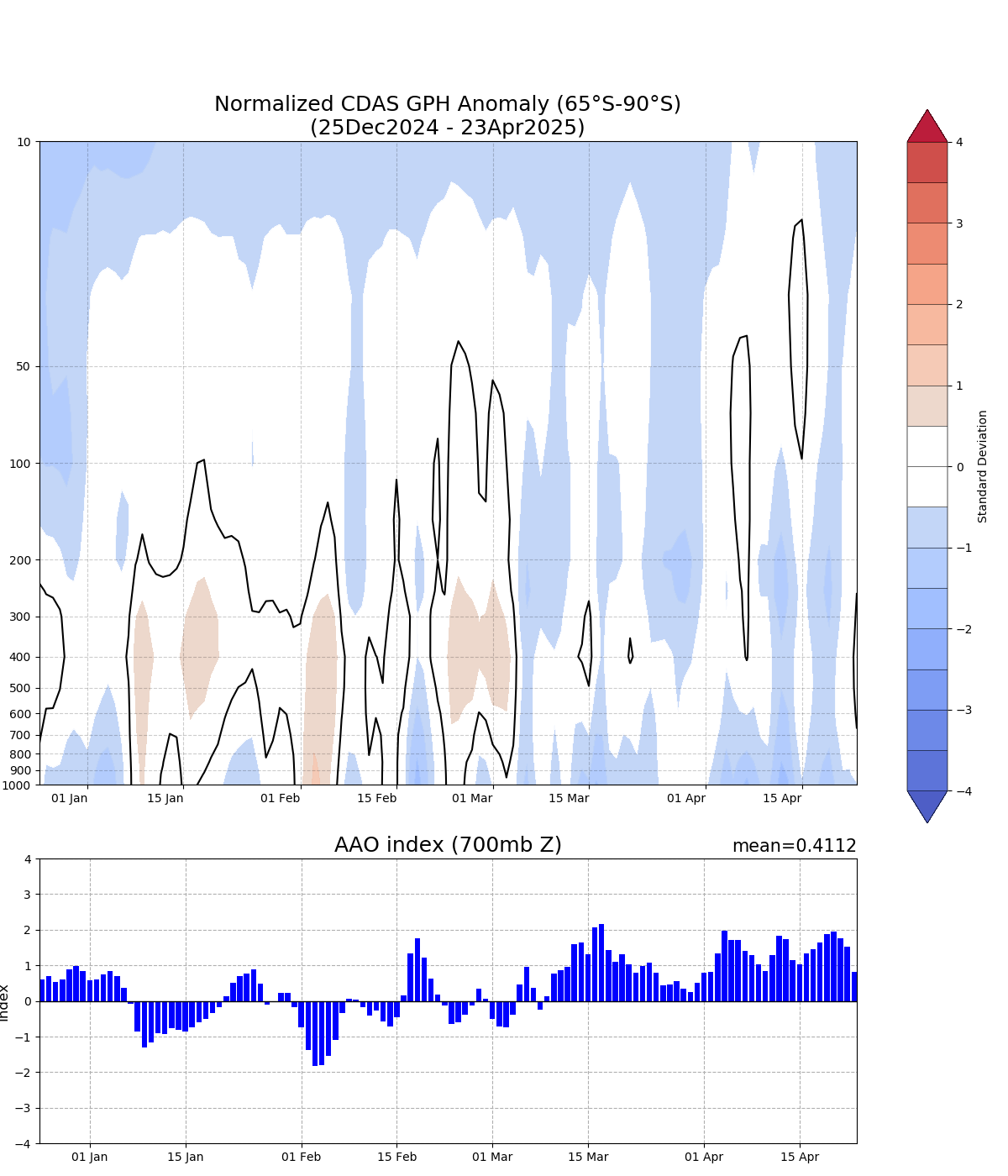
Vertical cross-section of geopotential height anomalies
The daily geopotential height anomalies at 14 pressure levels are shown for the previous
120 days as indicated, and they are normalized by standard deviation using 1979-2000 base period.
The anomalies are calculated by subtracting 1979-2000 daily climatology, and then averaged over the
polar cap poleward of 65°S.
The blue (red) colors represent a
strong (weak) polar vortex. The black solid lines show the zero anomalies.
The lower diagram shows the AAO index calculated daily.
Credits: cpc.ncep.noaa.gov